Traffic Sign Classifier

10 min readMay 5, 2021

To build this classifier, I used GTSRB — German Traffic Sign Recognition Benchmark dataset.

The German Traffic Sign Benchmark is a multi-class, single-image classification challenge held at the International Joint Conference on Neural Networks (IJCNN) 2011. We cordially invite researchers from relevant fields to participate: The competition is designed to allow for participation without special domain knowledge. Our benchmark has the following properties:

Single-image, multi-class classification problem
More than 40 classes
More than 50,000 images in total
Large, lifelike database

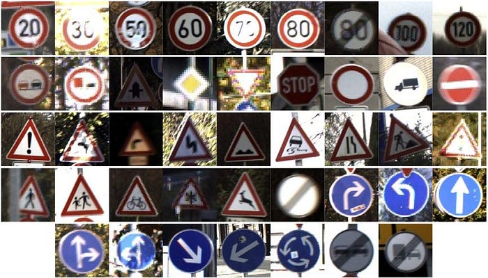
The German Traffic Sign Recognition Benchmark (GTSRB) contains 43 classes of traffic signs, split into 39,209 training images and 12,630 test images. The images have varying light conditions and rich backgrounds.

These are different types of classes which are present in dataset.

Training an image classifier

We will do the following steps in order:

Importing Libraries
Define a Convolutional Neural Network
Define a loss function
Train the network on the training data
Test the network on the test data

Importing libraries

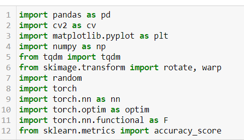
I have used many libraries to develop this classifier. I have used some new libraries like tqdm, skimage for better visualizations.

I have used cv2 package which is helpful to read images.

I have used torch which is a python library to develop neural networks architecture.

Pandas is a library which is used to load and read data

Dataset Visualization

Add paths where train and test data set is present.

To get a better view at the data let’s plot a bar plot using following code

It would gives us below plot

From above plot we can say that the dataset does not contain equal number of different class images. we can see there are classes like speed 20,dangerous curve, pedestrians , go straight and end of passing which have less than 100 images. Comparatively , classes like keep right, speed limit 30, speed limit 50 and yeild which had more than 700 images per class. So we might not get better accuracy for classes with less images.

For Increasing dataset size and to made dataset generic, later in this project we use image augmentation.

Let’s take a look at what this csv file contains.

width, height is the image dimensions. Class id columns to indicate to which class this particular image belongs. Path is where the image is present. Roi is pixel values of rectangular box of image.

We will use classid and path for this project

Loading Dataset

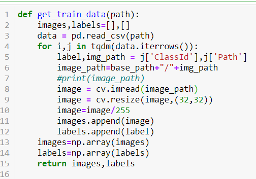
Using this user defined function I have loaded dataset.

I have used cv library to read image and resize it.

tqdm is the library to show the progress bar.

we have loaded 39209 train and 12630 test images.

Image Augmentation

The problem with classifiers is that we cannot train a better classifier with small dataset. So, to increase our dataset size we use techniques like image augmentation.

Image augmentation is a process of generating new images. We create these new images from the images we already have.

We have used rotation, flipup and flipdown transformations for images.

There are several other transformations to use like shear, normalization. I cannot apply all transformation techniques as i am programming on medium end laptop.

Let’s take a loot at shape after we image augmentation.

As you can see, after image augmentation our dataset size has increased from 39209 to 156836.

Let’s split our train data set into train and validation datasets using.

We have splitted our train data set into train and validation dataset with 20% for validation dataset.

Let’s take a look at images.

Subplot is a function of matplot lib which allows us to plot graphs at row and column wise.

Now we need to convert our lists into tensors and respective data types.

Developing Model

As we have enough dataset, I have decided to develop a neural network model for classification instead of other available classifiers.

To develop a good classification model in neural network. We need to know about Convolution neural networks, Max pool , drop layers and batch normalization.

Convolution Neural networks

In a CNN, the input is a tensor with a shape: (number of inputs) x (input height) x (input width) x (input channels).

After passing through a convolutional layer, the image becomes abstracted to a feature map, also called an activation map, with shape: (number of inputs) x (feature map height) x (feature map width) x (feature map channels).

For example if an image of size 32*32 with 3 channels are passed to convolution layer with window size of 3, we would get image of 30*30 with 3 channels.

if we send the image to cnn layer with window size 5 we would get image of 28*28.

A convolutional layer within a CNN generally has the following attributes:

Convolutional filters/kernels defined by a width and height (hyper-parameters).
The number of input channels and output channels (hyper-parameters). One layer’s input channels must equal the number of output channels (also called depth) of its input.
Additional hyperparameters of the convolution operation, such as: padding, stride, and dilation.

Maxpooling

Pooling layers reduce the dimensions of data by combining the outputs of neuron clusters at one layer into a single neuron in the next layer.

Max pooling uses the maximum value of each local cluster of neurons in the feature map

for example if we send an image of 32*32 to a maxpool layer of size 2*2, we would get output as 16*16 image.

Dropout Layers

Dropout layers are used to prevent model from overfitting. It is a regularization method. It works by dropping or ignoring some nodes in the model during training.

It can be applied on dense layers, convolution layers and recurrent layers.

Batch Normalization

It is a technique used for standardizing the inputs of the layers in mini-batches. This helps in stabilizing the learning process and reduces number of epochs required to train model.

Using these layers, I have developed below model.

CUDA is a parallel computing platform and application programming interface model created by Nvidia. It allows software developers and software engineers to use a CUDA-enabled graphics processing unit for general purpose processing

Cross Entropy Loss

Cross entropy loss also known as log loss uses in classification models when the output is between 0 or 1.

It uses following formula

−(ylog(p)+(1−y)log(1−p))

Adam Optimizer

Adam optimizer is mix of RMSprop and SGD withmomentum.It uses the squared gradients to scale the learning rate like RMSprop and it takes advantage of momentum by using moving average of the gradient instead of gradient itself like SGD with momentum.

Training

we train the model with 10 epochs with batch sizes of 32.

Below are the progress bars which shows it’s time and progress in mean time.

Here we are saving the trained model for future reference. So that we don’t have to start from beginning.

Let’s see how loss decreases over epochs.

Let’s see how this model works on validation dataset.

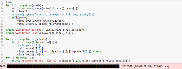
We are getting accuracy of 0.79 with loss of 0.655

Let’s check accuracy of specific classes on validation dataset.

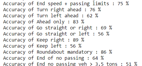
Let’s see how this model is working on test dataset.

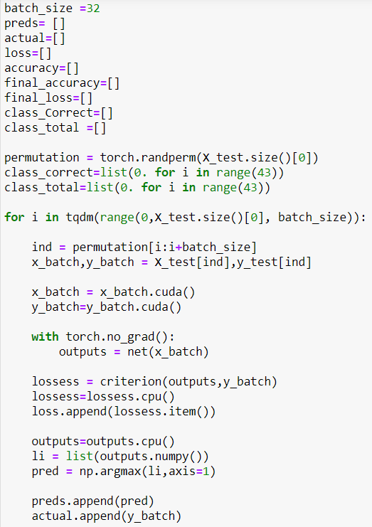
We got accuracy of 71% with 0.9 loss.

Let’s check accuracy of specific classes on Test dataset.

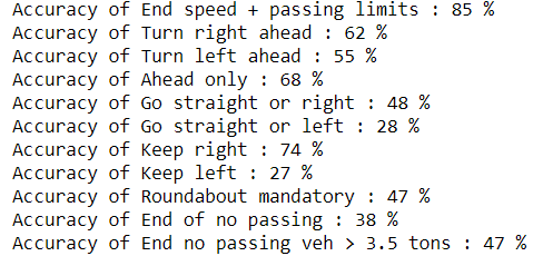
From accuracy of specific classes, we can see that the accuracy of classes speed 20, double curve, dangerouls curve left, dangerous curve right, pedestarins, beaware of ice et.,has less than 50%.

This is because of data size. Earlier we have seen that data size of these specific classes are less than others.